Using Mean And Mean Absolute Deviation To Compare Data Iready
So, I was at my nephew's birthday party the other day, right? Chaos, as usual. Tiny humans zipping around, sugar levels through the roof. Anyway, his mom, bless her heart, was trying to figure out if she'd bought enough juice boxes for the inevitable beverage drought. She'd done some kind of mental calculation, mumbling about "average thirst" and "how many kids usually drink two." It was… a process. And honestly, it got me thinking. How do we really know if one group of numbers is "better" or "more consistent" than another? Especially when you're dealing with stuff like… well, learning data. Like the kind you see on iReady.
You know that feeling, right? You log into your iReady dashboard (or maybe you're a teacher staring at a sea of student progress reports) and you see all these numbers. Scores, time spent, proficiency levels. And then you're supposed to make sense of it all. Are the students in Class A learning more than Class B? Is this new intervention really making a difference, or is it just a fluke? It's enough to make you want to hide behind the nearest pile of party balloons. But fear not, dear reader! We're about to dive into a couple of handy tools that can shed some light on this numerical jungle: the mean and the mean absolute deviation.
Think of it this way: the mean is like that simple, everyday answer everyone asks for. "What's the average score?" "What's the typical amount of time spent?" It's your go-to, your first instinct. But is it enough? Sometimes, the mean can be a little… misleading. Like if you're comparing the salaries of a small tech startup. You might have a couple of founders raking in millions, and then a whole bunch of junior developers making a much more modest wage. The mean salary might look ridiculously high, but it doesn't really tell the story of what most people are actually earning, does it? That's where our trusty sidekick, the mean absolute deviation, swoops in to save the day.
The Mean: Our Familiar Friend (Mostly)
Let's start with the mean. You probably know this one already. It's the average. You add up all the numbers in a set and then divide by how many numbers there are. Simple, right?
Imagine we have two groups of students, Group X and Group Y, and we're looking at their scores on a recent math assessment.
Group X Scores: 75, 80, 85, 90, 95
Group Y Scores: 60, 70, 80, 90, 100
To find the mean for Group X, we add them up: 75 + 80 + 85 + 90 + 95 = 425. Then we divide by 5 (because there are 5 scores): 425 / 5 = 85.
For Group Y, we add: 60 + 70 + 80 + 90 + 100 = 400. And divide by 5: 400 / 5 = 80.
So, right off the bat, it looks like Group X has a slightly higher average score. That's pretty straightforward. The mean tells us the central tendency, the "typical" score if you will, for each group. It's like the party mom's "average thirst" calculation – a good starting point.
But here's where it gets interesting. What if we had another group, Group Z?
Group Z Scores: 10, 70, 80, 90, 170
Let's calculate the mean for Group Z. Add them up: 10 + 70 + 80 + 90 + 170 = 420. Divide by 5: 420 / 5 = 84.
Now, look at that! Group Z has a mean score of 84, which is very close to Group X's mean of 85. Based on the mean alone, you might think Group X and Group Z are performing pretty similarly. But are they really? Take a peek at those scores. Group X has scores clustered pretty tightly around the mean: 75, 80, 85, 90, 95. They're all within 10 points of the average. Group Z, on the other hand, has scores all over the place: a 10, a 70, an 80, a 90, and a whopping 170! That 170 is pulling the average up, but it doesn't represent the typical performance of most students in that group. It's like having one super-genius who gets 100% and everyone else struggles to pass. The mean score might be decent, but the reality is a lot more varied.
This is the classic limitation of the mean. It's sensitive to outliers – those extreme values that can skew the results. So, while the mean is super useful for giving us a general idea, it doesn't tell us anything about the spread or variability of the data. And in education, especially with something as complex as learning, that spread is crucial.
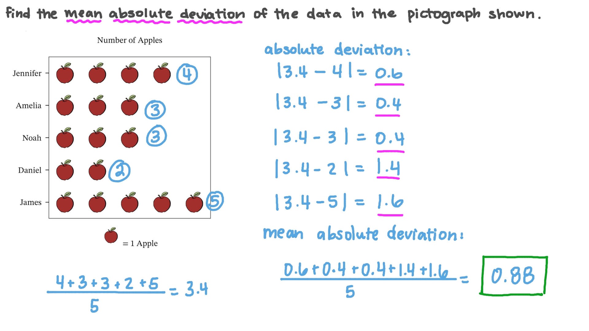
Enter the Mean Absolute Deviation: The Unsung Hero of Consistency
This is where our friend, the Mean Absolute Deviation (MAD), comes in. Its name might sound a bit like a tongue twister, but its purpose is beautifully simple: it measures how much, on average, each data point deviates (or is different) from the mean. In plainer English, it tells us how spread out our data is.
Think of it like this: if the MAD is small, it means most of your data points are clustered close to the mean. This suggests consistency. If the MAD is large, it means your data points are spread out far from the mean, indicating more variability. It's like comparing two dart boards. One has all the darts clustered tightly around the bullseye (low MAD), and the other has darts scattered all over the board (high MAD). Both might have the same average distance from the bullseye (mean), but one is clearly more precise.
Let's go back to our groups. We already know the means:
Group X Mean: 85
Group Y Mean: 80

Group Z Mean: 84
Now, let's calculate the MAD for each group. Remember, "absolute" means we ignore the negative signs. We're just interested in the distance from the mean.
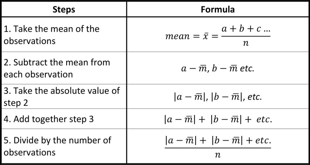
Calculating the MAD: Step-by-Step (Don't Worry, It's Not Scary!)
We'll use Group X's scores again: 75, 80, 85, 90, 95. And their mean is 85.
1. Find the difference between each score and the mean:
- 75 - 85 = -10
- 80 - 85 = -5
- 85 - 85 = 0
- 90 - 85 = 5
- 95 - 85 = 10
2. Take the absolute value of each difference (get rid of the minus signs):
- |-10| = 10
- |-5| = 5
- |0| = 0
- |5| = 5
- |10| = 10
3. Add up these absolute differences:
10 + 5 + 0 + 5 + 10 = 30
4. Divide by the number of scores (which is 5):
30 / 5 = 6
So, the Mean Absolute Deviation for Group X is 6. This means, on average, the scores in Group X are about 6 points away from the mean of 85.
Now, let's do the same for Group Y (scores: 60, 70, 80, 90, 100; mean: 80):
- |60 - 80| = |-20| = 20
- |70 - 80| = |-10| = 10
- |80 - 80| = |0| = 0
- |90 - 80| = |10| = 10
- |100 - 80| = |20| = 20
Sum of absolute differences: 20 + 10 + 0 + 10 + 20 = 60
MAD for Group Y: 60 / 5 = 12
And for Group Z (scores: 10, 70, 80, 90, 170; mean: 84):
- |10 - 84| = |-74| = 74
- |70 - 84| = |-14| = 14
- |80 - 84| = |-4| = 4
- |90 - 84| = |6| = 6
- |170 - 84| = |86| = 86
Sum of absolute differences: 74 + 14 + 4 + 6 + 86 = 184
MAD for Group Z: 184 / 5 = 36.8
Putting It All Together: The Real Story
Let's look at our findings:
- Group X: Mean = 85, MAD = 6
- Group Y: Mean = 80, MAD = 12
- Group Z: Mean = 84, MAD = 36.8
Suddenly, the picture changes, doesn't it?
We initially thought Group X and Group Z were performing similarly because their means were close (85 vs. 84). But when we look at the MAD:
- Group X has a low MAD (6), meaning their scores are clustered tightly around the mean. This indicates a high level of consistency. Most students are performing at a similar level.
- Group Z has a very high MAD (36.8). This tells us that their scores are spread out considerably from the mean. The outlier of 170 is a big contributor here. It suggests a lot of variability, with some students doing exceptionally well and others struggling significantly.
- Group Y has a MAD of 12. This is higher than Group X, indicating more spread, but significantly lower than Group Z.
So, if your goal is to see if a group is generally performing at a certain level with minimal variation, Group X looks like the clear winner. If you're looking at a group where there's a wide range of performance, Group Z might be what you're seeing. The MAD helps you understand the shape of the data, not just its center.
In the context of iReady data, this is gold! As a teacher, you might be looking at two different intervention groups. Both might have a similar average improvement in their math scores (the mean). But if one group has a low MAD, it means the intervention is working consistently for most students. If the other group has a high MAD, it might be that the intervention is a huge success for a few students but not helping others as much, or even hindering them. That's a crucial distinction for deciding what to do next, right? You can't just rely on the average!
It's like comparing two playlists. Playlist A has 10 songs that are all upbeat pop. Playlist B has 5 slow ballads and 5 heavy metal tracks. Both playlists might have the same "average tempo" (if such a thing existed!), but they feel and sound very different. The MAD is the musical equivalent of "genre consistency."
Why This Matters for iReady (and Life!)
Understanding both the mean and the MAD gives you a more nuanced picture. It allows you to:
- Identify outliers: A high MAD can signal the presence of extreme values that might warrant further investigation. Are they data entry errors? Or are they genuine performance spikes or dips that need attention?
- Assess consistency: A low MAD indicates that the data points are similar to each other. This is often desirable in educational settings, suggesting that learning is happening at a relatively uniform pace.
- Compare groups more effectively: You can now compare groups not just on their average performance, but also on their variability. This is essential for understanding the impact of interventions or instructional strategies.
- Make more informed decisions: Whether you're a teacher adjusting instruction, a student aiming for specific goals, or even that party mom trying to ensure enough juice boxes, having a clearer understanding of your data leads to better choices.
So next time you're staring at those iReady reports, don't just skim the averages. Take a moment to consider the spread. The mean tells you where the center is, but the mean absolute deviation tells you how spread out the story is. And often, it's the story of the spread that holds the most valuable insights. It’s like the difference between knowing the average speed of cars on a highway and knowing if all the cars are going roughly the same speed or if there are a lot of really fast and really slow ones. Both are useful, but the latter paints a much clearer picture of the traffic conditions.
It's a bit like that anecdote about the party mom. She might have figured out the "average thirst," but she probably didn't account for the kid who inhales three juice boxes before anyone else even gets one, or the one who nurses a single sip for the entire party. Those variations, those deviations from the average, are what make things interesting (and sometimes chaotic!). And by understanding the MAD, we can start to get a handle on those variations, whether they're related to juice boxes or student learning.
So go forth, embrace the mean and the mean absolute deviation, and unlock a deeper understanding of your data. Your iReady reports (and maybe even your future party planning!) will thank you for it. It's really not as complicated as it sounds, and it opens up a whole new world of data interpretation. Happy analyzing!